Today we’re talking about the neuron, which is the basic building block of artificial neural networks. So let’s get started. Previously we saw an image

which looked like this. And these are actual, real-life neurons that have smeared onto glass, colored a little bit, and are observed through a microscope. So this is what they look like as you can see, quite an interesting structure. A body, and a lot of different tails, kind of branches coming out of them. And this is very interesting but the question is how can we recreate that in a machine? Because we really need to recreate that in a machine since the whole purpose of Deep Learning is to mimic how the human brain works. In the hopes that by doing so, we are going to create something amazing. We are going to create an amazing infrastructure for machines to be able to learn. And why do we hope for that? Well because the human brain is, well just happens to be one of the most powerful learning tools on the planet, or like learning mechanisms on the planet. And we just hope that if we recreate that we’ll have something as awesome as that. So our challenge right now, our very first step to creating artificial neural networks, is to recreate a neuron. So how do we do that? Well, first let’s take a closer look at what it actually is.

This image was first created by a Spanish neural scientist, Santiago Ramón y Cajal, in 1899. And what he did was he dyed neurons in actual brain tissue and looked at them under a microscope. And while he was looking at them he actually drew what he saw. And this is what he saw. He saw two neurons or two large neurons over there at the top, which had all these branches coming out of them towards their top parts, and then each had a rod or thread coming out towards the bottom, a very long one. And that’s what he saw. And now, you know, technology has advanced quite a lot and we have seen neurons much closer and more detailed and now we can actually draw what it looks like diagrammatically.

So let’s have a look at that. Here’s a neuron, this is what it looks like. Very similar to what Santiago Ramón drew over here. Here in this neuron what we can see is that it's got a body, that’s the main part of the neuron. And then its got some branches at the top, which are called dendrites. And its also got an axon, which is the long tail of the neuron. So what are these dendrites for and what’s the axon for? Well, the key point to understand here is that neurons by themselves are pretty much useless. It’s like an ant. An ant on its own can’t do much, like 5 ants together maybe they can pick something up. But again, they can’t build an anthill, they can’t establish a colony, they can’t work together as a huge organism. But at the same time, when you have lots and lots of ants like you have a million ants, they can build a whole colony, they can build an anthill. Same thing with neurons. By itself, it’s not that strong, but when you have lots of neurons together, they work together to do magic. And how do they work together? That’s a question. Well, that’s what the dendrites and axons are for. So the dendrites are kind of like the receivers of the signal for the neuron, and the axon is the transmitter of the signal for the neuron.

And here’s an image of how it all works conceptually. So at the top, you got a neuron, and you can see that its dendrites are connected to axons of other neurons that are even further away above it. And then the signal from this neuron travels down its axon and connects or passes onto the dendrites of the other neuron. And that’s how they’re connected. And in that small image over there, you can see that the axon doesn’t actually touch the dendrite. (laughs) A lot of machine learning, or a few machine learning scientists are very adamant about the fact that it doesn’t touch. It doesn’t touch, it has been proven that there is no physical connection there. But the point that we are interested in is that that connection between them, that the whole concept of the signal being passed, that’s called the synapse.

You can see over there, in that little image, that figure bracket is the synapse. That’s the term we’re going to be using. Instead of calling our artificial neurons, the lines we’re gonna have, or the connectors for artificial neurons we’re not be calling them axons or dendrites because then the question is whose connection is this? Is it that neuron’s or is it this neurons? We’re just going to call them synapses. And that kind of just answers all the questions. I mean it’s basically just where the signal is passed. Doesn’t matter who that element belongs to. That’s just a representation of the signal being passed and we see that just now. So basically that’s how a neuron works. Let’s move on to how we’re going to represent neurons or how we’re going to create neurons in machines.
So now we’re moving away from neural science and moving into technology. And here we go. So, here’s our neuron, also sometimes called the node. The neuron gets some input signals. And it has an output signal.
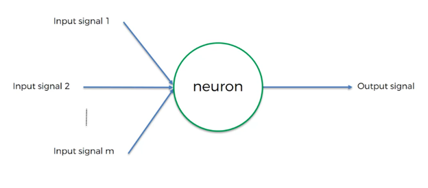
So dendrites and axons, remember? But again, we’re gonna call these synopses. These input signals, we’re going to represent them with other neurons as well. So, in this specific case, you can see that this neuron, this green neuron, is getting signals from yellow neurons. And in this course, we are going to try to stick to a certain color coding regime, where yellow means an input layer.
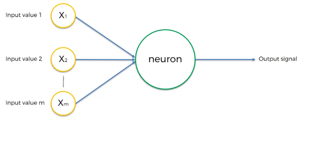
So basically all the neurons that are on the outer layer, on the first front of where the signals coming in. By signal, it might be a bit of an overkill to call this a signal. It’s just basically input value. So you know how even like in a simple linear regression you have input values, and then you have a predicted value. Same thing here. So you have input values, and there they are the yellow ones. And on the right to you we see just now it’ll be red, it’ll be the output value. The thing that I wanted to point out here is that in this specific example we are looking at a neuron that is getting its signals from the input layer neurons. So they are also neurons but they are input layer neurons. Sometimes you’ll have neurons that get their signal from other hidden layer neurons, so from other green neurons. And the concept is gonna be exactly the same. Just in this case, for simplicity’s sake, we’re portraying this example. And in terms of the input layer, the way to think about it is in the analogy of the human brain, the input layer is your senses, right. So whatever you can see, hear, feel, touch or smell. And of course, there’s a lot of things you can see, there’s a lot of information coming in. But those are your… that’s what your brain is limited to, it’s pretty much a (laughs) it’s pretty much lives in a box made out of bones and it’s only… It’s a mind-blowing fact to think about. Your brain is just locked in a black box, and the only thing… and it can’t see, it can’t hear, the only thing it’s getting is electrical impulses coming from these organs that you have, which are called your ears, nose, eyes, your sense of touch and whatever… and your taste. It’s just getting signals but it basically lives in this dark black box and it’s making sense of the world through your senses. It’s phenomenal. So you have these inputs that are coming in, and in terms of the human brain those are your five senses, in terms of machine learning or deep learning, that is basically your input values, so your independent variables, and we will get to that in a second. So your input values, the signal is passed through synapses to your neuron, and then your neuron has an output value, that passes further on down the chain. In this specific case, in terms of color coding, again yellow means input layer. So we kind of simplifying everything here. We’re saying we’re only gonna have like the input layer, then we’re gonna have one hidden layer, with the green, which is a hidden layer, and then we’re gonna have our output layer right away. So just so that we can get used to those colors for now. So there we go, that’s the basic structure. So now let’s look at a bit more detail at these different elements that we have. So we got the input layer. And what do we have here? Well, we have these inputs which are in fact independent variables.
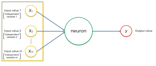
So independent variable one, independent variable two, and independent variable m. The important thing to remember here is that these independent variables are all for one single observation. So think of it as one row in your database. One observation. You just take all of the independent variables, maybe it’s the age of the person, the amount of money in their bank account, how do they drive or walk to work, what method of transportation do they use. But that’s all descriptions of one specific person, that you are, either you’re training your model on, or you’re performing some prediction on. And the other thing you need to know about these variables is that you need to standardize them.
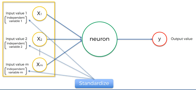
You need to either standardize them which means make sure they have a mean of zero and variance one, or you can also sometimes and Hadelin will point out these tricks in a bit more detail, perhaps in the practical tutorials you might come across these, sometimes you might want to not standardize you might wanna normalize them. Meaning that instead of making sure that the mean is zero and the variance is one, you just subtract the minimum value, and then you divide it by maximum minus minimum, so by the range of your values and therefore you get values between zero and one. Depend on the scenario you might wanna do one or the other but basically, you want all of these variables to be quite similar, in about the same range of values. Why’s that? Well, all of these values are going to go into a neural network whereas we all see just now they will be added up and multiplied by weights added up and so on. It’s just going to be easier for the neural network to process them if they are all about the same. And that’s just how it is going to be able to work properly. And if you want to read more about standardization, normalization and other things you can do with your input variables, a good additional reading paper is called Efficient BackProp by Yan LeCun 1998, the link’s over there. So Yan LeCun, we’re actually going to talk about this phenomenal person in the place of Deep Learning in the part of the course where we’re talking about illusional neural networks. You’ll see that this is definitely a person who knows what he’s talking about. He’s a close friend of Geoffrey Hinton, who we have already seen, who we’ve already mentioned. So in this paper, you will learn more about standardization and normalization. But you can pick up lots of other different tips and tricks and be a good source of additional reading as you go through this course. So check it out if you’re interested in some additional reading. There we go, so that’s what we need to do with the variables. And here we’ve got the output value. So what can our output value be?
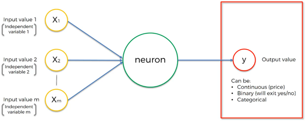
Well, we’ve got a couple of options. Output value can be, it can be continuous, for instance, price; it can be binary, for instance, a person will exit or stay, or it can be a categorical variable. If it’s a categorical variable, the important thing to remember here is that in that case, your output value won’t be just one, it’ll be several output values because these will be your dummy variables, which will be representing your categories. And that’s just how it works. Just important to remember that, in that case, that’s how you’re going to be getting your categories out of the artificial neural network. But let’s go back to our simple case of one output value. And now one more point, a point I’ve already made, I just want to reiterate this point. On the left, you’ve got a single observation, so one row from your data set, and on the right, you have a single observation as well. That is the same observation. So important to remember that whatever inputs you’re putting in, that’s for one row, and then the output you get back is for that exact same row. Or if you’re training your neural network then you’re putting the inputs in for that one row, you’re putting the output in for that one row. So if you wanna simplify the complexity, think of it as a simple linear regression, or a multi-variant linear regression. So you’re putting in your values, you have your output. There’s no question about it when we are talking about things like regression because we’re so used to it. Same thing here. It’s nothing too complex. We’re just putting in values, we’re getting output. But just remember that every time it’s one row that you’re dealing with. So you don’t get confused and start putting in like thinking these are different rows that you’re putting into your artificial neural network or something. This is all just values in that one row. So different observation, different characteristics of, or attributes relating to that one observation. Every single time. Okay, so the next thing that we wanna talk about here is the synapses.
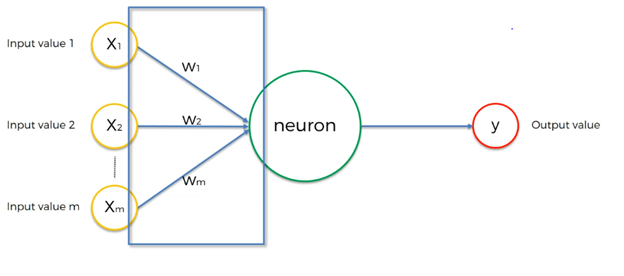
Here we’ve got synapses and they all actually get assigned weights. We’re gonna talk more about weights further down, but in short, weights are crucial to artificial neural networks functioning. Because weights are how neural networks learn. By adjusting the weights, the neural network decides in every single case, what signal is important and what signal is not important to a certain neuron, what signal gets passed along and what signal doesn’t get passed along, or to what strength, to what extent signals get passed along. So weights are crucial, they are the things that get adjusted through the process of learning. When you’re training your artificial neural network, you’re basically adjusting all of the weights in all of the synapses across this whole neural network and that’s where gradient descent and backpropagation come into play and those are concepts that we’ll also discuss. So basically those are the weights. That’s all you need to know for now. Here we’ve got the neuron. So signals go into the neuron and what happens in the neuron? So this is the interesting part. We’re talking about the neuron today, what happens inside the neuron? So, a few things happen. The first thing, and the first step is that all of these values that it’s getting, get added up.
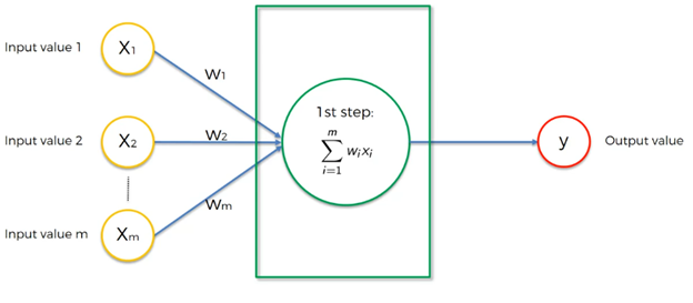
So it takes the added, so the weighted sum of all of the input values that it’s getting. Very simple, right? It’s very very straightforward. Just add up, multiply by the weight, add them up. And then, it applies an activation function.
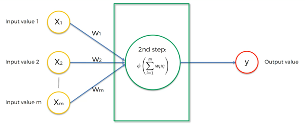
Now we’re gonna talk more about activation function further down but it’s basically a function that is assigned to this neuron or to this older, and it is applied to this weighted sum, and then from that, the neuron understands if it needs to pass on a signal. That’s the signal it passes on, the function applied to, the weighted sum. But basically depending on the function, the neuron will either pass on the signal or it won’t pass the signal on. And that’s exactly what happens here in step three. The neuron passes on that signal to the next neuron down the line.
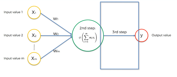
And that’s what we’re going to talk about in the next tutorial because it is quite an important topic. We want to delve deeper into the activation function. But hopefully, for now, everything is, should be pretty clear, how you’ve got input values, you’ve got weights, you’ve got these synapses, you’ve got something that happens in the neuron, you’ve got weighted sum and then the activation function applied to them that is passed on then that is repeated throughout the whole neural network, on and on and on and on.
Thousands of hundreds of thousands of times depending on how big, how many neurons you have, how many synapses you have in your neural network. So there we go! Hope you enjoyed today’s tutorial, can’t wait to see you next time. And until then, enjoy Deep Learning!

0 Comments
Post a Comment